March 2022 — This section explains how demographic data can be used to better understand the current and potential residents of your downtown. Demographic and lifestyle data can give you a starting point for an in-depth analysis of specific business and real estate development opportunities. This data also can help the broader community understand how it is changing.
Does your trade area population include more homeowners or renters? Baby Boomers, Gen-Xers, or Millenials? Which ethnic groups are represented in the population? If they are home owners, how likely are they to purchase home furnishings, renovate their homes, or spend leisure-time landscaping their yards?
To analyze market opportunities for your downtown, you need to examine data and ask questions like the above about residents of your trade area. This data must include the number of residents, as well as their household characteristics. Current and projected demographic, lifestyle and consumer spending data about your trade area from secondary sources can provide this information.
Demographic Data
It is well understood that product preferences vary across different groups of consumers. These preferences relate directly to consumer demographic characteristics, such as household type, income, age, and ethnicity. For this reason, it is not only the amount of demand that truly matters to a local economy. The mix of consumers also has a major impact on a local economy, and therefore must be thoroughly examined in all trade area analyses. Unfortunately, an enormous amount of data is readily available from a variety of private and public sources, leaving the reader with tables and tables of demographic information overload.
Relevant Data Categories
Interpretation of demographic data is often missing in market analysis. What does the data say about how the market is changing and how consumers spend their time and money? Specifically, what does the data suggest about new business or real estate opportunities downtown? The following provides a starting point in your understanding and interpretation of demographic data in relation to retail spending.
- Population and household data allow you to quantify the current market size and extrapolate future growth. Population is defined as all persons living in a geographic area. Households consist of one or more persons who live together in the same housing unit—regardless of their relationship to each other (this includes all occupied housing units). Households can be categorized by size, composition, or their stage in the family life cycle. Typically, demand is generated by the individual or the household as a group. The entire family influences a household purchase, such as a computer or TV. Individual purchases, on the other hand, are personal to the consumer. Anticipated household or population growth may indicate future opportunities for a retailer. An analysis of household and/or overall population growth provides the big picture of potential retail demand in a community. Further analysis is necessary to identify retail preferences within a community.
- Household income data is a good indicator of residents’ spending power. Household income positively correlates with retail expenditures in many product categories. When evaluating a market, retailers look at the median or average household income in a trade area and will seek a minimum number of households within a certain income range before establishing a business or setting prices. Another common practice is to analyze the distribution of household incomes. Discount stores may avoid extremely high or low-income areas. Some specialty fashion stores target incomes above $100,000. A few store categories, such as auto parts, are more commonly found in areas with lower household incomes. See the following box for more details on household income. Remember, though, that using income as the sole measure of a market’s buying preferences can be deceptive. You need to consider all categories of demographic data when analyzing a market.
- High-income households with annual incomes above $150,000 are the fastest growing segment of the U.S. population, nearly doubling between 2010 and 2020 (increase of 91 percent) and now account for 15 percent of all households. These households have more disposable income for high-end retail, fine dining, and cultural amenities such as museums and concert halls.
- Middle-income households with annual incomes between $50,000 and $150,000 are also growing, from 43 percent of households in 2010 to 46 percent in 2020. These households are more mindful of their expenses and tend to be more frugal and selective in their buying behavior.
- Low-income households with annual incomes below $50,000 are are shrinking and have decreased from 48 percent of all households in 2010 to 39 percent in 2020 as more households move up to higher income levels. These households spend most of their income on essentials such as housing, transportation, and groceries.
- Age is an important factor to consider because personal expenditures change as people age. Some things remain the same. AARP’s 2021 Home and Community Preferences Survey asked adults of all ages what makes a good community. Access to grocery stores, health care providers, safe parks, trails and streets, and opportunities for community engagement top the list. The 2021 survey found that over three quarters of adults age 50 and older want to remain in their homes as they age. This has remained consistent over time and suggests that this population will continue to support retailers and require services as they age. Consumer spending on drug stores and assisted care services flourish in areas with a large population of elders. In general, elders tend to spend less on goods and services. Areas popular with young families are well suited for toy stores, day care centers, and playgrounds. Arcades, clothing stores, and fast food restaurants are popular with teenagers. Some entertainment and recreational venues, such as movie theaters and golf courses, serve a broad section of the population.
- Occupational concentrations of white and blue-collar workers are used as another gauge of a market’s taste preferences. Specialty apparel stores thrive in middle to upper income areas and those with above-average white-collar employment levels. Second-hand clothing stores and used car dealerships are successful in areas with a higher concentration of blue-collar workers. Office supply stores and large music and video stores are especially sensitive to the occupational profile. These retailers target growth areas with a majority of white-collar workers.
- Housing ownership and rate of housing turnover is an important factor for numerous retailers to consider. Home ownership directly correlates with expenditures for home furnishings and home equipment. Furniture, appliances, hardware, paint/wallpaper, floor covering, garden centers and other home improvement products all prosper in active housing markets.
Comparing the Primary Trade Area with Other Areas
Demographic statistics are especially useful if they are presented in comparison with other places. To see how your trade area differs from other places, it is useful to provide two comparison sets of data: comparable communities and the state or U.S. as a whole.
Comparing your trade area with other communities and the state allows demographic baselines to be established. These baselines will help determine whether your trade area has low, median, or high values in each demographic category. For instance, after examining demographics for your trade area, it may appear that there is a high proportion of white-collar workers. However, this observation cannot be verified until you know what constitutes an average number of white-collar workers.
Comparable communities can include five or six cities of similar size in the same region or state. The cities chosen should reflect similar distances from metropolitan statistical areas (MSAs) of the region. The comparison cities should have a trade area of similar geographic size as your primary trade area.
In addition to comparable communities, adding state or U.S. statistics will provide a broader benchmark for comparing your community. State and U.S. data will include a blend of urban and rural areas. Accordingly, it will not be limited to similar places. However, differences between the trade area and the state or U.S. (such as per capita income) will be used later in your analysis of retail or service business opportunities.
Demographic Data Sources
Detailed local census data is readily available free via the Internet through the U.S. Bureau of Census. Census data can be retrieved at several geographic levels (county, city/village, census tract, zip code, etc.). The U.S. Census website includes a link to its user-friendly data-filled website. The site includes tools to view, print, and download statistics about population, housing, industry, and business. It also includes Census Bureau products, maps and visualizations.
In addition to the Census Bureau, there are numerous, nationally recognized data firms that can provide demographic estimates for a particular trade area. While much of these firms’ data is based on the U.S. Census and other public sources, they add value by providing annual updates. They also package the data in user-friendly comparative formats that make it easy to compare one geographic area with another. Furthermore, you are able to tap into the knowledge of skilled demographers who have designed data products centered on particular industry needs. These firms offer direct downloading of the data using their software. Prices charged by these firms have become more and more affordable as competition has increased.
Following is an example of a demographic comparison report assembled for a sample community from a private data source. The “subject trade area” column reflects demographics data on the trade area. The “comparable communities” column reflects the demographic averages of five or six other places and the “State” column provides a third level of comparison.
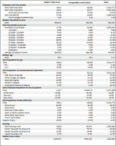
Sample Demographic Comparison Report
Lifestyle Data
Adding consumer lifestyle data takes the market analysis a step further. This data recognizes that the way people live (lifestyle) influences what they purchase as much as where they live (geography) or their age, income, or occupation (demography). Lifestyle data enables you to include people’s interests, opinions, and activities and the effect these have on buying behavior in our analysis.
Theory behind Lifestyle Segmentation
In his 2010 paper “Who Benefits Whom in the Neighborhood: Demographics and Retail Product Geography,” Joel Waldfogel examines the relationship between a community’s lifestyle characteristics and its product preferences. He concludes that retail is stimulated by large concentrations of populations of similar characteristics and tastes. As a result, a community can develop product mixes targeted to specific high-potential customer segments.
Concentrations of lifestyle segments create demand for specific products or services. This tendency to cluster is based on the premise that “birds of a feather flock together.” Did you ever notice that the homes and cars in any particular neighborhood are usually similar in size and value? If you could look inside the homes, you’d find many of the same products. Neighbors also tend to participate in similar leisure, social, and cultural activities.
The quality of a segmentation system is directly related to the data that goes into them. High quality and useful systems allow you to predict consumer behavior. In a retail business targeting tourists, for example, the systems allow the business to identify products and services that appeal to this market segment. The usefulness of a segmentation system depends on how well the data incorporates lifestyle choices, media use, and purchase behavior into the basic demographic mix. This supplemental data comes from various sources, such as automobile registrations, magazine subscription lists, and consumer product-usage surveys.
Lifestyle Data Sources
Several private data firms offer lifestyle cluster systems. The firms use data from the U.S. Census and other sources to separate neighborhoods throughout the U.S. into distinct clusters. They utilize sophisticated statistical models to combine several primary and secondary data sources to create their own unique cluster profiles. Most models start with data from U.S. Census block groups that contain 300-600 households. In rural areas, the data is more typically clustered by zip code.
One example of a cluster system used in modern demographic analysis is ESRI’s Tapestry Segmentation. The system divides every U.S. neighborhood into one of 65 unique market segments based on socio-economic and demographic characteristics.
Sample Lifestyle Segment Summary
As an example, qualitative information provided by ESRI for its “College Towns” designation includes:
- Demographic: Most residents are between the ages of 18 and 34, and live in single-person or shared households. The racial profile is typically similar to the nation as a whole, with three-fourths of college town residents being white.
- Socioeconomic: Because many students only work part-time, the median household income ranks near the low end of ESRI’s measurements. Most of the employed residents work in the service industry, holding on-again, off-again campus jobs.
- Consumer Behavior: Convenience dictates food choices. With their busy lifestyles, residents in college towns frequently eat out at fast-food restaurants and pizza outlets during the week. Because many college students are new residents to a town, bedding, bath, and cooking products are popular purchases. Music and nightlife venues are extremely popular in college towns.
The Tapestry Segmentation also includes quantitative data, such as the purchase potential index that measures potential demand for specific products or services. The index compares the demand for each market segment with demand for all U.S. consumers and is tabulated to represent a value of 100 as the average demand. Values above 100 indicate residents are more likely to purchase that product or participate in the respective activity. Conversely, values below 100 indicate residents are less likely to purchase the given product. For example, an index of 120 means that the spending potential in the tapestry segment is 20 percent higher than the nation as a whole. Sample data for the “College Town” segment is as follows:
| Consumer Behavior | Index to U.S. |
| Buy books | 106 |
| Shop at convenience stores | 114 |
| Go to bars/clubs | 214 |
| Attend movies | 135 |
| Owns a van or minivan | 27 |
From this data, a clear picture of the important demographic, socioeconomic, and consumer behavior of residents in college towns emerges. ESRI’s Tapestry Segmentation system provides similarly useful information in all 65 unique market segments it identifies.
Other examples of segmentation systems include Experian’s Mosaic® USA and Claritas PRIZM.
Cautions Regarding Lifestyle Segmentation
Lifestyle segmentation generalizes the types of customers in your trade area, which is helpful in making sense of a complex market. This simplification, however, may not fully capture the particular traits of your customer base or may overlook the richness of groups in your area. Furthermore, since data are not continually updated, lifestyle segments are based on a snapshot in time. This works well if social and economic conditions remain constant; however, significant changes may make the segment less representative of reality. Therefore, although lifestyle segments can greatly help you understand customers in your trade area, you should take care not to place too much weight on segmentation systems. Instead, regard the information as a part of the mix of demographic data.
Spending Potential Data
Estimates of household spending give a sense of the size of a market in dollars. For example, secondary data are available that allow you to estimate the size of the local food or restaurant market, based on the number of households in your trade area. Private data are also available to provide refined estimates based on local demographics. It is important to remember that these estimates measure the amount of spending by households residing in your trade area, not necessarily spending within your trade area that also includes non-residents. Conversely, residents of your trade area may choose to spend outside your trade area.
Consumer Expenditure Survey
The two-part Consumer Expenditure (CEX) Survey is the primary data source for spending-potential estimates that covers a whole range of household spending from dining to travel expenditures. The Bureau of Labor Statistics conducts the survey of American households continuously throughout the year and has been doing so since 1980. The results of the survey provide a comprehensive snapshot of household spending and are used to revise the important Consumer Price Index (CPI), which significantly influences both national markets and policy.
The CEX survey includes a Diary Survey of daily purchases and an Interview Survey of general purchases over time. The Diary Survey reflects record-keeping by consumer units (individual and household shoppers) for two consecutive week periods. This component of the CEX collects data on small, daily purchases that could be overlooked by the quarterly Interview Survey. The Interview Survey collects expenditure data from consumers in five interviews conducted every three months. The data from both surveys is integrated to provide a comprehensive database on all consumer expenditures.
Private Data Providers
Although the Consumer Expenditure Survey data alone provides valid and reliable estimates for your market, some private data companies refine the CEX survey data for more sophisticated estimates that may prove useful.
For example, ESRI uses Tapestry Segmentation lifestyle segments (see above), together with CEX data to estimate household spending. A conditional probability model links spending by the consumers surveyed to all households with similar socioeconomic characteristics. The results are spending estimates based on the demographics of a particular trade area, which are reported together with the average spending per household and a spending- potential index. The index compares the spending of the trade area’s households to the national average (see the following Sample Spending Potential Report).
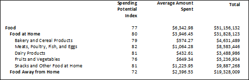
Sample Spending Potential Report
Using GIS to Analyze Your Market
Demographic analysis is useful in understanding purchasing characteristics for different market segments. While demographics can be collected and analyzed without the use of geographic information systems, GIS often aids and enhances the analysis. Since most downtown professionals may not be experts in GIS, you will probably want to enlist consultants, planners and/or marketing data providers to offer technical mapping assistance. Following are two examples of using GIS to assist in demographic analysis.
Using GIS to Visualize Trade Area Demographics
Demographic data for a trade area are often reported as single values for each demographic category. For example, the trade area income is reported as one value, even though income can vary across the trade area. GIS, however, can display demographic values in finer detail by geographic unit (zip code, census block group, etc.). Mapping these variations may reveal valuable, visual information that can be used to show the attractiveness of a downtown location and aid in business recruitment and expansion.
Effective demographic mapping requires an understanding of some basic cartographic concepts. Perhaps the most important concept is an understanding of the problems associated with demographic densities. By nature, downtown population density is usually higher than a similar-sized area on a community’s fringe. Moreover, many business owners would view the large concentration of customers as a competitive advantage over a non-downtown location. However, a map showing the number of people in each geographic unit (e.g. census block group) does not always show this relationship.
As a real world example of this problem, consider the following of the La Crosse, Wisconsin, area depicting the population by census block group. Why does this type of map fail to accurately represent the number of customers in downtown? The problem is that the sizes of census block groups differ. While the U.S. Census Bureau tries to control the number of households in each block group, it is not always possible to make the units the same size. Problems associated with geographical barriers (rivers, mountains, etc.), the nature of population distribution (sparse or concentrated), and household size can cause wide variations in geographic sizes and population numbers in census block groups.
As a result, census block groups covering large geographic areas tend to dominate the viewer’s eye on a map. When these large census block groups are located away from downtown, it appears that downtown has a small population compared to the outlying urban areas. Additionally, there may be many more block groups with smaller populations located in a smaller area. However, their small size and small population values can become obscured on a map. Consequently, the larger number and grouping of these smaller block groups need to be addressed. GIS can tackle this problem by creating a map that accurately depicts population density.
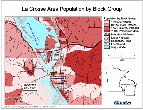
Sample Map Showing Population by Block Group
The following map illustrates the same La Crosse, Wisconsin, area with an equivalent color scheme. However, this new map has undergone a transformation and now accurately depicts the area’s population density. Here, the viewer sees that there is a large population clustered around the downtown and a relatively small population toward the urban fringes. The story told by the population density map would not be seen in a single population value representing the entire trade area. As a result, the new map aids in showing the potential of downtown as a business location and can be used as a valuable business recruitment tool.
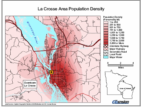
Sample Map Showing Population Density
Using GIS to Analyze Visitor Demographics
The previous section discussed how GIS could create a useful visual representation of demographics. However, GIS is not limited to producing maps and graphics. GIS can also be used as an analytical tool in demographic analysis. As an example, consider the problematic nature of assembling demographics for non-local visitors. Profiling visitors is essential in the study of tourists, commuters and other market segments. While collecting demographics for the surrounding resident market is a straightforward process, visitors can come from a wide area. Obtaining and analyzing demographics for every area that produced a visitor is unrealistic using traditional methods. In these instances, GIS can be used to profile demographics of the non-local market.
Many businesses dependent on visitors, such as hotels, maintain customer address lists. These addresses are useful in market analysis because knowing where visitors live provides information about their neighborhood demographics. What’s more, starting with a visitor’s address, GIS can be used to quickly identify the census block group, or neighborhood, where a customer lives. Each census block group is accompanied by rich demographic information available through the U.S. Census Bureau or through private data providers. Specifically, each census block group, or neighborhood, includes information on income, population, occupation, education, age and housing. This information can be entered into a GIS and used as a surrogate for demographic information on each individual visitor.
Using this neighborhood demographic information as a surrogate is based on the premise that “birds of a feather flock together.” As discussed in the section on lifestyle segmentation systems, people with similar demographics tend to live near one another. Therefore, the demographics of a neighborhood as a whole can be used to represent the demographics of an individual visitor from that neighborhood. Using addresses, GIS can determine every neighborhood that produced a visitor and extract the demographics of these neighborhoods. The demographics extracted from each visitor neighborhood can be combined to produce a useful demographic profile of the visitor market.
The demographic profile is even more useful when it is given some perspective. Similar to the comparable communities analysis discussed earlier in this section, the visitor demographic profile can be used to determine what makes visitors demographically different from the general population. Instead of comparing local community demographics to those of other communities, the visitor demographics can be compared to the demographics of a larger region. For instance, if visitors primarily originate from a three-state area, the visitor demographic profile can be compared to the demographics for the entire population of those three states. These demographic profiles of the community visitors and the larger region can be compared on a category by category basis.
The following example explains the steps used in GIS analysis of visitor demographics.
Step 1. GIS is used to map the locations of visitor addresses. As an example, the following shows a map of visitor origins for a sample community.
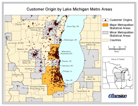
Sample Map Showing Place of Visitor Origin
Step 2. Once the visitor origins have been mapped, GIS is used to determine the neighborhoods containing each visitor and extract the associated neighborhood demographics. These neighborhood demographics are used as a surrogate for the demographics of an individual visitor. The following is a map of one sample neighborhood showing visitor origins, as well as some of the demographics associated with the neighborhood.
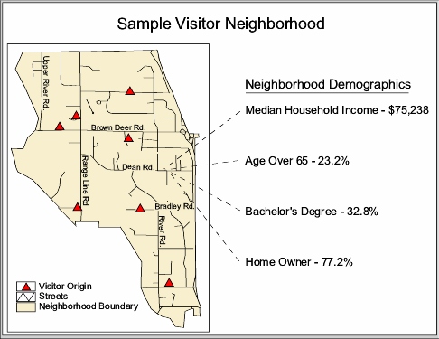
Sample Map Showing Neighborhood and Demographic Attributes
Step 3. GIS is used to combine all of the demographics extracted from every visitor neighborhood. Combining the neighborhoods creates a demographic profile of the visitors. To aid in the analysis, GIS also creates a demographic profile of the larger region. The regional demographic profile includes every neighborhood in the region instead of just those neighborhoods that produced visitors. These two profiles are then used to examine differences in visitor demographics. For instance, the table shown below compares several demographic categories. The first column contains the demographic category; the second column shows the visitor demographic profile; and the third column depicts the profile created for the larger region. In this example, GIS was able to demonstrate that visitors originated in neighborhoods that had higher incomes, a greater proportion of college-educated residents, more executive and professional employees, a higher rate of home ownership, and more vehicles per household than the overall three-state region.
Sample Table Comparing Demographics of Visitor Neighborhoods Compared to Region
| Demographic Category | Demographic Visitor Profile | Demographic Regional Profile |
| Males | 48.7% | 48.9% |
| Females | 51.3% | 51.1% |
| Average Household Size | 2.6 | 2.5 |
| Median Age | 36.5 | 36.5 |
| Age Less Than 18 | 25.4% | 26.7% |
| Age 16 or More | 77.3% | 76.2% |
| Age 25 Or More | 66.6% | 64.1% |
| Age 65 or More | 12.6% | 12.9% |
| Median Household Income | $48,231 | $37,561 |
| Average Household Income | $60,973 | $40,302 |
| Per Capita Income | $21,564 | $15,694 |
| Education: High School | 20.0% | 21.5% |
| Education: Some College | 12.4% | 11.3% |
| Education: Associate Degree | 4.4% | 4.4% |
| Education: Bachelor’s Degree | 13.1% | 7.6% |
| Education: Graduate Degree | 7.1% | 4.1% |
| Occupation: Executive | 15.4% | 11.2% |
| Occupation: Professional | 17.8% | 13.8% |
| Occupation: Technician | 3.6% | 3.6% |
| Occupation: Sales | 13.3% | 11.2% |
| Occupation: Clerical | 15.9% | 16.1% |
| Occupation: Services | 9.6% | 12.5% |
| Occupation: Production | 9.4% | 11.1% |
| Home Owner | 75.1% | 67.3% |
| Home Renter | 24.9% | 32.7% |
References:
White, J.R., & Gray, K.D. (Eds.). (1996). Shopping centers and other retail properties: Investment, development, financing and management. Hoboken, NJ: John Wiley & Sons.
Waldfogel, J. (2010). Who benefits whom in the neighborhood? Demographics and retail product geography. In Glaeser, E.L. (Ed.), Agglomeration economics (pp.181-209). Cambridge, MA: National Bureau of Economic Research.
Binette, Joanne. 2021 Home and Community Preference Survey: A National Survey of Adults Age 18-Plus. Washington, DC: AARP Research, November 2021. https://doi.org/10.26419/res.00479.001
About the Toolbox and this Section
The 2022 update of the toolbox marks over two decades of change in our small city downtowns. It is designed to be a resource to help communities work with their Extension educator, consultant, or on their own to collect data, evaluate opportunities, and develop strategies to become a stronger economic and social center. It is a teaching tool to help build local capacity to make more informed decisions.
This free online resource has been developed and updated by over 100 university educators and graduate students from the University of Wisconsin – Madison, Division of Extension, the University of Minnesota Extension, the Ohio State University Extension, and Michigan State University – Extension. Other downtown and community development professionals have also contributed to its content.
The toolbox is aligned with the principles of the National Main Street Center. The Wisconsin Main Street Program was a key partner in the development of the initial release of the toolbox. One of the purposes of the toolbox has been to expand the examination of downtowns by involving university educators and researchers from a broad variety of perspectives.
The current contributors to each section are identified by name and email at the beginning of each section. For more information or to discuss a particular topic, contact us.


 How to Utilize Data for Community Economic Development (Part II)
 How to Access Data for Community Economic Development (Part I)
 Developing Questions for Focus Group Interviews